About this vignette
This shows you how to take a dataset, fit a model, and apply tdmore to investigate predictive performance and precision dosing.
Source dataset
We will use a well-known example dataset: pheno.
##    ID  TIME  AMT  WT APGR   DV EVID MDV
## 1   1   0.0 25.0 1.4    7   NA    1   1
## 2   1   2.0   NA 1.4    7 17.3    0   0
## 3   1  12.5  3.5 1.4    7   NA    1   1
## 4   1  24.5  3.5 1.4    7   NA    1   1
## 5   1  37.0  3.5 1.4    7   NA    1   1
## 6   1  48.0  3.5 1.4    7   NA    1   1
## 7   1  60.5  3.5 1.4    7   NA    1   1
## 8   1  72.5  3.5 1.4    7   NA    1   1
## 9   1  85.3  3.5 1.4    7   NA    1   1
## 10  1  96.5  3.5 1.4    7   NA    1   1
## 11  1 108.5  3.5 1.4    7   NA    1   1
## 12  1 112.5   NA 1.4    7 31.0    0   0
## 13  2   0.0 15.0 1.5    9   NA    1   1
## 14  2   2.0   NA 1.5    9  9.7    0   0
## 15  2   4.0  3.8 1.5    9   NA    1   1
## 16  2  16.0  3.8 1.5    9   NA    1   1
## 17  2  27.8  3.8 1.5    9   NA    1   1
## 18  2  40.0  3.8 1.5    9   NA    1   1
## 19  2  52.0  3.8 1.5    9   NA    1   1
## 20  2  63.5   NA 1.5    9 24.6    0   0
## 21  2  64.0  3.8 1.5    9   NA    1   1
## 22  2  76.0  3.8 1.5    9   NA    1   1
## 23  2  88.0  3.8 1.5    9   NA    1   1
## 24  2 100.0  3.8 1.5    9   NA    1   1
## 25  2 112.0  3.8 1.5    9   NA    1   1
## 26  2 124.0  3.8 1.5    9   NA    1   1
## 27  2 135.5   NA 1.5    9 33.0    0   0
Building your model
We will fit a 1-compartment model to this dataset using nlmixr.
library(nlmixr)
library(tidyverse)
modelCode <- function() {
  ini({
    LTHETA2 <- log(50)
    LTHETA3 <- log(0.1)
    #variances
    ETA2 ~ 1
    ETA3 ~ 1
    EPS1 <- 0.1
  })
  model({
    LWT = log(WT / 70)
    V=exp(LTHETA2+LWT+ETA2)
    CL=exp(LTHETA3+LWT*0.75+ETA3)

    d/dt(centr) = -CL/V*centr
    CONC=centr/V
    CONC ~ add(EPS1)
  })
}

pheno_nlmixr <- pheno %>%
  nlmixr(modelCode, data=., est="focei")
Adapting the model for tdmore
An nlmixr model already contains both the structural model and the description of inter-individual variability and residual variability.
## Structural model: RxODE
##
## Parameters:
## name var cv
## ETA2 2 1.414214
## ETA3 1 1.000000
##
## Covariates: WT
##
## Residual error model:
## name type additiveError proportionalError
## CONC constant 0.1 0Alternatively, you can specify your model using RxODE or algebraic equations. In these cases, you have to specify the inter-individual variability and residual variability manually.
Performing a posthoc
Now that we have a model, we can perform a posthoc fit on retrospective data. We will first convert the dataset to tdmore format.
regimen <- pheno %>% filter(EVID==1) %>% select(ID, TIME, AMT)
observed <- pheno %>% filter(EVID==0 & MDV == 0) %>% transmute(ID, TIME, CONC=DV)
covariates <- pheno %>% select(ID, TIME, WT)
db <- dataTibble(object=m1, regimen, observed, covariates)
#We will only perform the evaluation for the first 5 subjects, for performance reasons
db <- db[1:5, ]And then perform a posthoc fit.
## # A tibble: 5 x 8
## # Rowwise:
## ID object regimen observed covariates fit elapsed ipred
## <int> <list> <list> <list> <list> <list> <list> <list>
## 1 1 <tdmor… <df[,2] [1… <df[,2] [2… <df[,2] [12 … <tdmor… <proc_ti… <df[,2]…
## 2 2 <tdmor… <df[,2] [1… <df[,2] [3… <df[,2] [15 … <tdmor… <proc_ti… <df[,2]…
## 3 3 <tdmor… <df[,2] [1… <df[,2] [3… <df[,2] [15 … <tdmor… <proc_ti… <df[,2]…
## 4 4 <tdmor… <df[,2] [1… <df[,2] [3… <df[,2] [14 … <tdmor… <proc_ti… <df[,2]…
## 5 5 <tdmor… <df[,2] [1… <df[,2] [3… <df[,2] [14 … <tdmor… <proc_ti… <df[,2]…You can plot a single fit from this easily using autoplot.
autoplot(posthocPrediction$fit[[1]], se.fit=FALSE)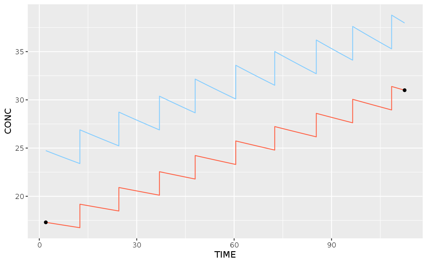
Quantifying prediction accuracy
Let us now explore how well we can predict future concentrations. Proseval creates a tibble with a fit per concentration.
## # A tibble: 6 x 9
## # Rowwise:
## ID object regimen observed covariates fit elapsed ipred OBS
## <int> <list> <list> <list> <list> <list> <list> <list> <dbl>
## 1 1 <tdmor… <df[,2] [… <df[,2] [… <df[,2] [12… <tdmo… <proc_t… <df[,2… 0
## 2 1 <tdmor… <df[,2] [… <df[,2] [… <df[,2] [12… <tdmo… <proc_t… <df[,2… 1
## 3 1 <tdmor… <df[,2] [… <df[,2] [… <df[,2] [12… <tdmo… <proc_t… <df[,2… 2
## 4 2 <tdmor… <df[,2] [… <df[,2] [… <df[,2] [15… <tdmo… <proc_t… <df[,2… 0
## 5 2 <tdmor… <df[,2] [… <df[,2] [… <df[,2] [15… <tdmo… <proc_t… <df[,2… 1
## 6 2 <tdmor… <df[,2] [… <df[,2] [… <df[,2] [15… <tdmo… <proc_t… <df[,2… 2We can use this data to plot how well we can predict the future for this population. The OBS variable describes how many previous concentrations are included in the fit.
prosevalResults %>%
unnest(cols=c(observed, ipred), names_sep=".") %>%
group_by(ID, OBS) %>% mutate(INCLUDED = row_number() <= OBS) %>%
ggplot(aes(x=ipred.TIME, y=ipred.CONC - observed.CONC)) +
geom_smooth(se=F) +
geom_hline(yintercept=0) +
geom_hline(yintercept=c(-1.96, 1.96)*m1$res_var[[1]]$sigma(), linetype=2) +
geom_point(aes(color=INCLUDED)) +
scale_x_continuous(breaks=seq(0, 999, by=24)) +
facet_wrap(~OBS, labeller=label_both)## `geom_smooth()` using method = 'loess' and formula 'y ~ x'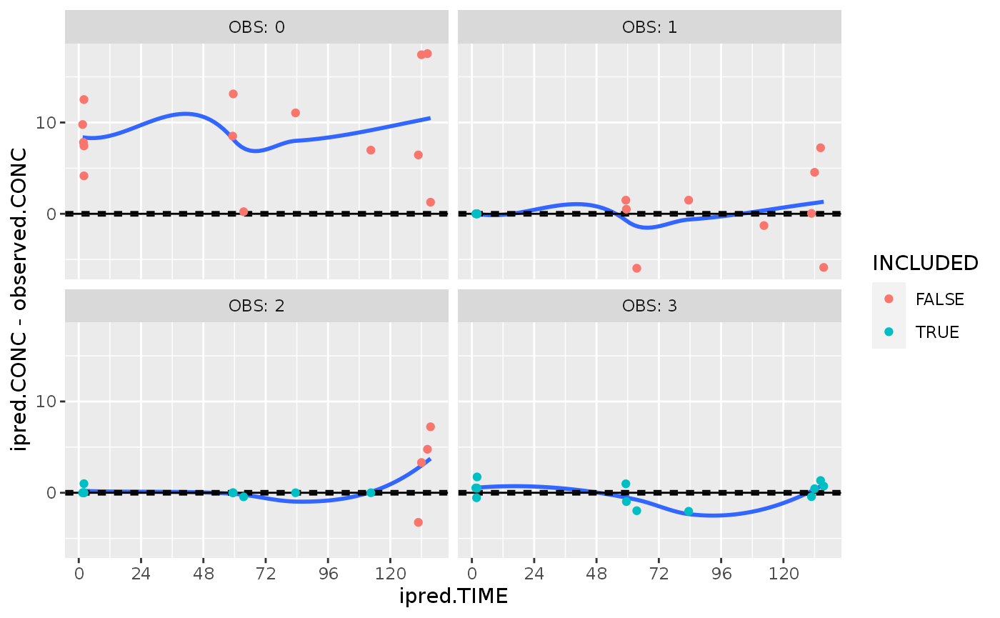
The concentration data early post-treatment is insufficient to accurately predict the future time course.
Exploring MIPD performance
We can now simulate precision dosing using this model.
## We need to add some metadata to the model to easily optimize
m2 <- m1 %>%
metadata(formulation("Default", "mg", dosing_interval=24)) %>%
metadata(target(min=30, max=30))
## The modified simulation database:
## keep ID, fit, and covariates
## the fit is used as the "truth" to predict new concentrations
## the new regimen assumes a default 24h-based administration
simulationDb <- posthocPrediction %>% ungroup() %>%
select(ID, fit, covariates) %>%
mutate(regimen=list(data.frame(TIME=seq(0, 140, by=24), AMT=NA, FORM="Default")),
object=list(m2))
## Adjustment option 1: measure at each trough
measureAtTrough <- function(fit, regimen, truth) {
if(nrow(fit$observed) == 0) {
rec <- findDoses(fit)
list(nextTime=regimen$TIME[2]-0.01, regimen=rec$regimen)
} else {
now <- max(fit$observed$TIME) + 3
regimen$FIX <- !(regimen$TIME > now)
rec <- findDoses(fit, regimen=regimen)
nextTime <- regimen$TIME[match(FALSE, regimen$FIX)] #next trough
list(nextTime=nextTime-0.01, regimen=rec$regimen)
}
}
## Adjustment option 2: measure 8h before trough, so you can still adapt
measure8hBeforeTrough <- function(fit, regimen, truth) {
if(nrow(fit$observed) == 0) {
rec <- findDoses(fit)
list(nextTime=regimen$TIME[2]-8, regimen=rec$regimen)
} else {
now <- max(fit$observed$TIME) + 3
regimen$FIX <- !(regimen$TIME > now)
rec <- findDoses(fit, regimen=regimen)
nextTime <- regimen$TIME[match(FALSE, regimen$FIX)+1] #next trough
list(nextTime=nextTime-8, regimen=rec$regimen)
}
}
## Adjustment option 3: rich profile at the beginning
richProfileAtBeginning <- function(fit, regimen, truth) {
richProfile <- c(1, 3, 4, 6, 8, 10)
if(nrow(fit$observed) == 0) {
rec <- findDoses(fit)
return( list(nextTime=richProfile[1], regimen=rec$regimen) )
}
nextTime <- richProfile[nrow(fit$observed) + 1]
regimen$FIX <- FALSE
regimen$FIX[1] <- TRUE #loading dose cannot be changed
if(nrow(fit$observed) == length(richProfile)) {
rec <- findDoses(fit, regimen=regimen)
regimen <- rec$regimen
}
list(nextTime=nextTime, regimen=regimen)
}
simulationResult <- doseSimulation(simulationDb, optimize=measureAtTrough) %>% mutate(method="A. At Trough")## Iteration # 0
## Iteration # 1
## Iteration # 2
## Iteration # 3
## Iteration # 4
## Iteration # 5
## Iteration # 0
## Iteration # 1
## Iteration # 2
## Iteration # 3
## Iteration # 4
## Iteration # 5
## Iteration # 0
## Iteration # 1
## Iteration # 2
## Iteration # 3
## Iteration # 4
## Iteration # 5
## Iteration # 0
## Iteration # 1
## Iteration # 2
## Iteration # 3
## Iteration # 4
## Iteration # 5
## Iteration # 0
## Iteration # 1
## Iteration # 2
## Iteration # 3
## Iteration # 4
## Iteration # 5
simulationResult2 <- doseSimulation(simulationDb, optimize=measure8hBeforeTrough) %>% mutate(method="B. 8h before trough")## Iteration # 0
## Iteration # 1
## Iteration # 2
## Iteration # 3
## Iteration # 4
## Iteration # 5
## Iteration # 0
## Iteration # 1
## Iteration # 2
## Iteration # 3
## Iteration # 4
## Iteration # 5
## Iteration # 0
## Iteration # 1
## Iteration # 2
## Iteration # 3
## Iteration # 4
## Iteration # 5
## Iteration # 0
## Iteration # 1
## Iteration # 2
## Iteration # 3
## Iteration # 4
## Iteration # 5
## Iteration # 0
## Iteration # 1
## Iteration # 2
## Iteration # 3
## Iteration # 4
## Iteration # 5
simulationResult3 <- doseSimulation(simulationDb, optimize=richProfileAtBeginning) %>% mutate(method="C. Rich profile")## Iteration # 0
## Iteration # 1
## Iteration # 2
## Iteration # 3
## Iteration # 4
## Iteration # 5
## Iteration # 6
## Iteration # 0
## Iteration # 1
## Iteration # 2
## Iteration # 3
## Iteration # 4
## Iteration # 5
## Iteration # 6
## Iteration # 0
## Iteration # 1
## Iteration # 2
## Iteration # 3
## Iteration # 4
## Iteration # 5
## Iteration # 6
## Iteration # 0
## Iteration # 1
## Iteration # 2
## Iteration # 3
## Iteration # 4
## Iteration # 5
## Iteration # 6
## Iteration # 0
## Iteration # 1
## Iteration # 2
## Iteration # 3
## Iteration # 4
## Iteration # 5
## Iteration # 6
fullResult <- bind_rows(simulationResult, simulationResult2, simulationResult3) %>%
group_by(ID, method) %>% filter(row_number() == n()) %>% #only keep the last regimen
mutate(ipred = purrr::map2(fit, next_regimen, ~predict(.x, regimen=.y, newdata=0:144)))
head(fullResult)## # A tibble: 6 x 12
## # Groups: ID, method [6]
## ID covariates regimen object observed iterationFit next_regimen OBS
## <int> <list> <list> <list> <list> <list> <list> <int>
## 1 1 <df[,2] [12… <df[,3] … <tdmor… <df[,6] … <tdmoreft> <df[,4] [6 … 5
## 2 2 <df[,2] [15… <df[,3] … <tdmor… <df[,6] … <tdmoreft> <df[,4] [6 … 5
## 3 3 <df[,2] [15… <df[,3] … <tdmor… <df[,6] … <tdmoreft> <df[,4] [6 … 5
## 4 4 <df[,2] [14… <df[,3] … <tdmor… <df[,6] … <tdmoreft> <df[,4] [6 … 5
## 5 5 <df[,2] [14… <df[,3] … <tdmor… <df[,6] … <tdmoreft> <df[,4] [6 … 5
## 6 1 <df[,2] [12… <df[,3] … <tdmor… <df[,6] … <tdmoreft> <df[,4] [6 … 5
## # … with 4 more variables: next_observed <list>, fit <list>, method <chr>,
## # ipred <list>The doseSimulation function has performed an iterative estimate - adapt routine. It uses nextTime to know when to simulate the next concentration sample, re-estimate the individual fit, and allow dose adaptation.
The final result is a dataset detailing every dose adaptation step. The final regimen can be found at the last line for each subject. We use this regimen to predict concentration from 0 to 150 hours. This can be used to show in silico dosing performance.
ggplot(fullResult, aes(x=TIME, y=CONC)) +
geom_line(data=. %>% unnest(cols=ipred), aes(group=interaction(method,ID), color=method)) +
geom_point(data=. %>% unnest(cols=observed)) +
geom_hline(yintercept=30, linetype=2) +
geom_hline(yintercept=30+c(1.96, -1.96)*m1$res_var[[1]]$add, linetype=2, alpha=0.3) +
theme(legend.position="none") +
facet_wrap(~method)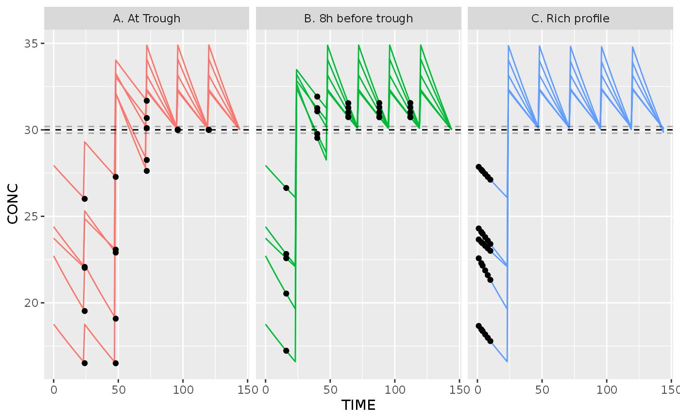
The dots in the above figure show simulated concentration samples, used to refine the individual fit. The lines are the resulting concentrations from the “true” fit.
Conclusion? For our simple example, simulations indicate measuring 8h before trough (strategy B) is the superior approach, as it reaches the target sooner with similar accuracy to measuring at trough (strategy A). Note that the high additive residual error of 0.1 limits the information obtained from each concentration sample.
Code appendix
set.seed(0)
library(ggplot2)
library(dplyr)
library(tidyr)
library(tdmore)
pheno %>% filter(ID %in% c(1,2))
library(nlmixr)
library(tidyverse)
modelCode <- function() {
ini({
LTHETA2 <- log(50)
LTHETA3 <- log(0.1)
#variances
ETA2 ~ 1
ETA3 ~ 1
EPS1 <- 0.1
})
model({
LWT = log(WT / 70)
V=exp(LTHETA2+LWT+ETA2)
CL=exp(LTHETA3+LWT*0.75+ETA3)
d/dt(centr) = -CL/V*centr
CONC=centr/V
CONC ~ add(EPS1)
})
}
pheno_nlmixr <- pheno %>%
nlmixr(modelCode, data=., est="focei")
m1 <- tdmore(pheno_nlmixr)
summary(m1)
regimen <- pheno %>% filter(EVID==1) %>% select(ID, TIME, AMT)
observed <- pheno %>% filter(EVID==0 & MDV == 0) %>% transmute(ID, TIME, CONC=DV)
covariates <- pheno %>% select(ID, TIME, WT)
db <- dataTibble(object=m1, regimen, observed, covariates)

#We will only perform the evaluation for the first 5 subjects, for performance reasons
db <- db[1:5, ]
posthocPrediction <- posthoc(db)
print(posthocPrediction)
autoplot(posthocPrediction$fit[[1]], se.fit=FALSE)
prosevalResults <- proseval(db)
head(prosevalResults)
prosevalResults %>%
  unnest(cols=c(observed, ipred), names_sep=".") %>%
  group_by(ID, OBS) %>% mutate(INCLUDED = row_number() <= OBS) %>%
  ggplot(aes(x=ipred.TIME, y=ipred.CONC - observed.CONC)) +
  geom_smooth(se=F) +
  geom_hline(yintercept=0) +
  geom_hline(yintercept=c(-1.96, 1.96)*m1$res_var[[1]]$sigma(), linetype=2) +
  geom_point(aes(color=INCLUDED)) +
  scale_x_continuous(breaks=seq(0, 999, by=24)) +
  facet_wrap(~OBS, labeller=label_both)
## We need to add some metadata to the model to easily optimize
m2 <- m1 %>%
  metadata(formulation("Default", "mg", dosing_interval=24)) %>%
  metadata(target(min=30, max=30))

## The modified simulation database:
## keep ID, fit, and covariates
## the fit is used as the "truth" to predict new concentrations
## the new regimen assumes a default 24h-based administration
simulationDb <- posthocPrediction %>% ungroup() %>%
  select(ID, fit, covariates) %>%
  mutate(regimen=list(data.frame(TIME=seq(0, 140, by=24), AMT=NA, FORM="Default")),
         object=list(m2))

## Adjustment option 1: measure at each trough
measureAtTrough <- function(fit, regimen, truth) {
  if(nrow(fit$observed) == 0) {
    rec <- findDoses(fit)
    list(nextTime=regimen$TIME[2]-0.01, regimen=rec$regimen)
  } else {
    now <- max(fit$observed$TIME) + 3
    regimen$FIX <- !(regimen$TIME > now)
    rec <- findDoses(fit, regimen=regimen)
    nextTime <- regimen$TIME[match(FALSE, regimen$FIX)] #next trough
    list(nextTime=nextTime-0.01, regimen=rec$regimen)
  }
}

## Adjustment option 2: measure 8h before trough, so you can still adapt
measure8hBeforeTrough <- function(fit, regimen, truth) {
  if(nrow(fit$observed) == 0) {
    rec <- findDoses(fit)
    list(nextTime=regimen$TIME[2]-8, regimen=rec$regimen)
  } else {
    now <- max(fit$observed$TIME) + 3
    regimen$FIX <- !(regimen$TIME > now)
    rec <- findDoses(fit, regimen=regimen)
    nextTime <- regimen$TIME[match(FALSE, regimen$FIX)+1] #next trough
    list(nextTime=nextTime-8, regimen=rec$regimen)
  }
}

## Adjustment option 3: rich profile at the beginning
richProfileAtBeginning <- function(fit, regimen, truth) {
  richProfile <- c(1, 3, 4, 6, 8, 10)
  if(nrow(fit$observed) == 0) {
    rec <- findDoses(fit)
    return( list(nextTime=richProfile[1], regimen=rec$regimen) )
  }

  nextTime <- richProfile[nrow(fit$observed) + 1]
  regimen$FIX <- FALSE
  regimen$FIX[1] <- TRUE #loading dose cannot be changed
  if(nrow(fit$observed) == length(richProfile)) {
    rec <- findDoses(fit, regimen=regimen)
    regimen <- rec$regimen
  }
  list(nextTime=nextTime, regimen=regimen)
}

simulationResult <- doseSimulation(simulationDb, optimize=measureAtTrough) %>% mutate(method="A. At Trough")
simulationResult2 <- doseSimulation(simulationDb, optimize=measure8hBeforeTrough) %>% mutate(method="B. 8h before trough")
simulationResult3 <- doseSimulation(simulationDb, optimize=richProfileAtBeginning) %>% mutate(method="C. Rich profile")
fullResult <- bind_rows(simulationResult, simulationResult2, simulationResult3) %>%
  group_by(ID, method) %>% filter(row_number() == n()) %>% #only keep the last regimen
  mutate(ipred = purrr::map2(fit, next_regimen, ~predict(.x, regimen=.y, newdata=0:144)))

head(fullResult)
ggplot(fullResult, aes(x=TIME, y=CONC)) +
  geom_line(data=. %>% unnest(cols=ipred), aes(group=interaction(method,ID), color=method)) +
  geom_point(data=. %>% unnest(cols=observed)) +
  geom_hline(yintercept=30, linetype=2) +
  geom_hline(yintercept=30+c(1.96, -1.96)*m1$res_var[[1]]$add, linetype=2, alpha=0.3) +
  theme(legend.position="none") +
  facet_wrap(~method)